高性能python-性能分析
这里是对 «Python高性能分析» 的文章解析。
将会引用来自书中的代码, 添加一些个人的理解备注, 作为学习笔记使用。
计算Julia集合
import time

x1, x2, y1, y2 = -1.8, 1.8, -1.8, 1.8
c_real, c_imag = -0.62772, -.42193
def calculate_z_serial_purepython(maxiter, zs, cs):
    """Calculate output list using Julia update rule"""
    output = [0] * len(zs)
    for i in range(len(zs)):
        n = 0
        z = zs[i]
        c = cs[i]
        while abs(z) < 2 and n < maxiter:
            z = z * z + c
            n += 1
        output[i] = n
    return output
def calc_pure_python(desired_width, max_iterations):
    ''' 获取两个常数数组, x从x1 到 x2 均匀递增, y从y2 到 y1 均匀递减'''
    x_step = (float(x2 - x1) / float(desired_width))
    y_step = (float(y1 - y2) / float(desired_width))
    x = []
    y = []
    ycoord = y2
    while ycoord > y1:
        y.append(ycoord)
        ycoord += y_step
    xcoord = x1
    while xcoord < x2:
        x.append(xcoord)
        xcoord += x_step
    ''' 为图像中的每个格子构建一个复数值 '''
    zs = []
    cs = []
    for ycoord in y:
        for xcoord in x:
            zs.append(complex(xcoord, ycoord))
            cs.append(complex(c_real, c_imag))

    print("Length of x:", len(x))
    print("Total elements:", len(zs))
    start_time = time.time()
    output = calculate_z_serial_purepython(max_iterations, zs, cs)
    end_time = time.time()
    secs = end_time - start_time
    print(calculate_z_serial_purepython.__name__ + " took", secs, "seconds")

    # This sum is expected for a 1000^2 grid with 300 iterations.
    # It catches minor errors we might introduce when we're
    # working on a fixed set of inputs.
    assert sum(output) == 33219980
calc_pure_python(desired_width=1000, max_iterations=300)
在以上这段代码中,可以看出函数的执行时间在 8s 左右。这里边有值得一提的是 我们可以通过装饰器构造一个方法来计算方法的执行时间。
就像下面这样。
from functools import wraps

def timefn(fn):
    @wraps(fn)
    def measure_time(*args, **kwargs):
        t1 = time.time()
        result = fn(*args, **kwargs)
        t2 = time.time()
        print ("@timefn:" + fn.func_name + " took " + str(t2 - t1) + " seconds")
        return result
    return measure_time
但不可避免的是,这样的方法总是要在源代码上添加一些代码,我们可以通过以下方法来获取一个函数的执行时间。
计算代码执行时长
我们可以通过几种办法获取一个函数的具体执行时长。
- python代码使用 timeit 模块这将会通过-n 执行循环次数, -r 指定重复次数,通过重复执行获取最好的结果
python -m timeit -n 5 -r 5 -s "<some code>"
- unix 下使用 time 命令这将会返回三个值, real 记录整体耗时, user 记录cpu在任务执行上消耗的时长, sys 记录cpu在调度过程内核函数消耗的时长
/usr/bin/time -p python "<file>"
这里可以通过添加参数 --verbose 获取更加详细的结果。
其中Major (requiring I/O) page faults指标表示 任务在磁盘IO上消耗的时长,这个值会造成user + sys = real的较大偏差
- ipython 下使用 %timeit 魔法命令
这个命令和 python 的 timeit 模块效果是一致的,区别是需要在 ipython 环境下执行
使用cProfile模块
我们可以通过以下命令来调用cProfile模块获得代码中的每个函数的调用统计。
这其中包括 Ncalls 调用次数, cumtime 函数耗时时长, tottime 函数内部没有调用函数的其他代码的耗时时长。
python -m cProfile -s cumulative -o profile.stats julia_nopil.py
-s cumulative 对函数时间进行排序
-o 输出文件, 可以通过以下命令读取统计文件import pstats p = pstats.Stats("profile.stats") p.sort_stats("cumulative") p.print_stats()
使用可视化工具对cProfile的输出进行可视化
有时候查看cProfile的文件还是太过麻烦,这时就可以通过相应的可视化工具进行输出,这样更加直观方便。
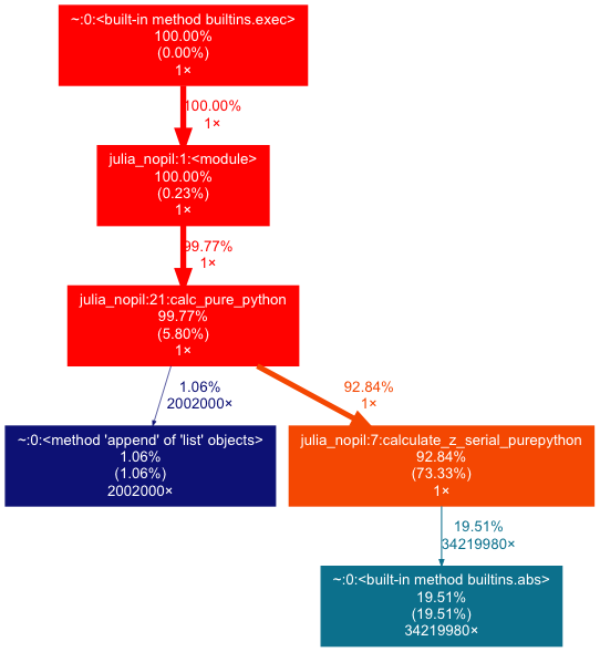
!python3 -m cProfile -s cumulative -o profile.stats julia_nopil.py
!gprof2dot -f pstats profile.stats | dot -Tpng -o ../../../images/high-performance-python/section-2/profile.png
得到下图. 从图中可以看出各个函数往下执行的调用占比。
!vprof -c c julia_nopil.py # 这里将会执行启动一个web server,在浏览器上展示分析的结果
使用LineProfiler进行逐行分析
在上文我们找到耗时占比较大的函数之后。就可以通过 line_profile 来进行逐行分析。
使用 pip install line_profiler安装模块之后。
我们需要修改代码文件。在需要分析的函数处添加装饰器 @profile
这里我们标记耗时较长的 calculate_z_serial_purepython 函数
!kernprof -l -v julia_lineprofiler.py
从上面的输出看出,主要消耗时间集中在 while 循环中。
while判断 甚至两行赋值语句,都因为循环了 34219980次 而导致占比时间均在 30%左右。
while 判断中是两个表达式,无从判断两个表达式何者占用的时间更慢
但是通过推导可知,函数会比单纯的逻辑表达式更慢。
在while表达式之后,我们可以通过调整 两个表达式的先后顺序,使得第一次判断的时间减少
理论上将优化一定的性能,而书中的结果也印证了这一点在对整体对函数
calc_pure_python分析中,引用书上的结果,
calculate_z_serial_purepython占用了97%的时间,可见创建列表的耗时在此次无足轻重
分析内存用量
书上提到了使用memory_profiler 分析的方法,但是在实际生产环境中, memory_profiler会导致代码的执行效率急剧降低,这是不可忍受的。
好在我们可以通过Ipython的 %memit 来分析 某些语句的 RAM使用情况。
这些内容将会在后续章节中说明。
单元测试
!cat ex.py
对上述代码进行单元测试
!nosetests ex.py
Comments !